Linux Layer 3 Cisco Router and Open vSwitch with NetFlow Virtualization

Configuring Cisco and Open Switch Routers and Layer 3 devices to send NetFlow data to a Linux NTOP NetFlow collector to interpret higher layer network flows.

Introduction

Layer 2 and Layer 3 Linux Switching (using kernel-supported utilities) is fast and efficient.  Open vSwitch -- when combined with an OpenFlow controller -- is a full-blown Software Defined Networking (SDN) implementation that offers the advantages of offloading topology and switching decisions to a centralized controller, allowing the Open vSwitch devices to primarily switch frames instead of expending processor and memory resources on topology maintenance and decision-making.
Open vSwitch devices are also Layer 3 and above aware, able to modify traffic based upon Layer 3 (IP address) and Layer 4 (TCP port) information.  However, an administrator needs quality information to make prioritization and routing decisions and OpenFlow controllers provide mostly Layer 2 information.  Systems monitoring devices -- MRTG, Cacti, Munin, Nagios/Icinga and Zabbix -- operate primarily at the device level (e.g. interface utilization, interface errors, interface congestion) and are difficult, if not impossible, to configure for detailed analysis.  Firewalls and access lists operate at the requisite levels (Layers 2, 3 and 4) for detailed traffic analysis, but require a great deal of manual configuration and interpretation to characterize traffic.
The term used for this kind of detailed traffic characterization is Flows.  Each flow has unique end devices, IP addressing and TCP ports.  At the flow level, each step in the path between end devices (i.e. intermediary switches and routers) also records traffic.  As stated above, OpenFlow controllers report this quite well at Layer 2.  Other protocols, such as NetFlow and OpenFlow, provide the higher-level information required to more precisely characterize and manage traffic.

Configuring Open vSwitch Layer 3 Switching

There are several ways to implement Layer 3 functionality, such as fake bridges and VLANs.  From a monitoring perspective, these can be somewhat problematical because they do not appear in SNMP MIBs.

This article will use multiple bridges on each Layer 3 Open vSwitch to define multiple networks.  Bridge and port membership is defined with the ovs-vsctl set of commands.  IP address assignments to the bridges is managed at boot time in the /etc/network/interfaces file.  Routing is managed using Quagga.

In the topology at the top of the article, there is routing configured on the Cisco R1 gateway and Open vSwitch devices Switch-01 and Switch-05.  All are members of OSPF Area 10.128.0.0 (range 10.128.0.0/13 with configured networks 10.128.0.0/24 and 10.128.1.0/24) and the Cisco router is also a member of the host laptop's Backbone Area 0.0.0.0 (range 172.16.0.0/12).

Switch-01 Configuration

The /etc/network/interfaces File

auto eth0
iface eth0 inet manual

auto eth1
iface eth1 inet manual

auto eth2
iface eth2 inet manual
...
auto eth7
iface eth7 inet manual

auto br0
iface br0 inet static
    address 10.128.0.254
    netmask 255.255.255.0
    network 10.128.0.0
    broadcast 10.128.0.255
    gateway 10.128.0.1
    # dns-* options are implemented by the resolvconf package, if installed
    dns-nameservers 192.168.1.1
    dns-search mydomain.com

auto br1
iface br1 inet static
    address 10.128.1.254
    netmask 255.255.255.0
    network 10.128.1.0
    broadcast 10.128.1.255
    # dns-* options are implemented by the resolvconf package, if installed
    dns-nameservers 192.168.1.1
    dns-search mydomain.com

Open vSwitch Configuration

18ce5ab3-d025-49c2-8cd8-0a41d3927c79
    Bridge "br1"
        Controller "tcp:10.128.0.102:6633"
            is_connected: true
        Port "eth4"
            Interface "eth4"
        Port "br1"
            Interface "br1"
                type: internal
    Bridge "br0"
        Controller "tcp:10.128.0.102:6633"
            is_connected: true
        Port "eth1"
            Interface "eth1"
        Port "eth6"
            Interface "eth6"
        Port "eth5"
            Interface "eth5"
        Port "eth3"
            Interface "eth3"
        Port "br0"
            Interface "br0"
                type: internal
        Port "eth7"
            Interface "eth7"
        Port "eth2"
            Interface "eth2"
        Port "eth0"
            Interface "eth0"
    ovs_version: "2.1.3"

The Quagga OSPF Configuration

router ospf
 ospf router-id 10.128.0.254
 network 10.128.0.0/24 area 10.128.0.0
 network 10.128.1.0/24 area 10.128.0.0
 area 10.128.0.0 range 10.128.0.0/13

Switch-05 Configuration

The /etc/network/interfaces file

auto eth0
iface eth0 inet manual

auto eth1
iface eth1 inet manual

auto eth2
iface eth2 inet manual
...
auto eth7
iface eth7 inet manual

auto br0
iface br0 inet static
    address 10.128.1.250
    netmask 255.255.255.0
    network 10.128.1.0
    broadcast 10.128.1.255
    # dns-* options are implemented by the resolvconf package, if installed
    dns-nameservers 192.168.1.1
    dns-search mydomain.com

Open vSwitch Configuration

18ce5ab3-d025-49c2-8cd8-0a41d3927c79
    Bridge "br0"
        Controller "tcp:10.128.0.102:6633"
            is_connected: true
        Port "eth1"
            Interface "eth1"
        Port "eth6"
            Interface "eth6"
        Port "eth0"
            Interface "eth0"
        Port "eth5"
            Interface "eth5"
        Port "eth3"
            Interface "eth3"
        Port "br0"
            Interface "br0"
                type: internal
        Port "eth4"
            Interface "eth4"
        Port "eth7"
            Interface "eth7"
        Port "eth2"
            Interface "eth2"
    ovs_version: "2.1.3"

The Quagga OSPF Configuration

router ospf
 ospf router-id 10.128.1.250
 network 10.128.1.0/24 area 10.128.0.0
 area 10.128.0.0 range 10.128.0.0/13

Installing NTOP on Ubuntu 14.04 Trusty Tahr

Keep in mind NTOP is not NTOP-NG.  NTOP-NG is the current version of the utility, but it decouples NetFlow from the application and requires the paid nProbe package.  For this article, we will use the older -- but still useful -- original NTOP.

The Easy (and Broken) Way

It's very easy -- apt-get install ntop.  You will need to configure the listening interface(s) and supply an administrator password.

The problem with this installation is the package does not install the visualization packages required for elements like pie graphs and host details, despite using the last version (5.0.1 dated 2012-08-13).  The package does not provide the full range of ntop features.

Compiling from Source

Install dependencies

sudo apt-get install libpcap-dev libgdbm-dev libevent-dev librrd-dev python-dev libgeoip-dev automake libtool subversion

sudo apt-get build-dep ntop 

Extract and compile

tar zxvf ntop-5.0.1.tar.gz
cd ntop-5.0.1
./autogen
make
sudo make install

Copy libraries to the correct location, change ownership of the executable and restart the service

sudo cp /usr/local/lib/libntop* /usr/lib/
sudo chown -R ntop.ntop /usr/local/share/ntop
sudo service ntop restart

Configuring NTOP

The installation process specifies one or more listening interfaces.  These are available without additional configuration.  The overview report provides information about this (ese) interface(s), such as packet distribution and size.

 There is also a tab for protocol distribution.

 

 And another for Application Protocols.

In a switched environment, an interface in promiscuous mode will still only capture unicast traffic switched to its own port, broadcast and multicast traffic.  The capture does not reflect overall network activity.

One option to capture traffic is port mirroring, in which all traffic on a specified interface is forwarded to another (in this case, the NTOP monitor).  The drawbacks to port mirroring are manual configuration, the added bandwidth and processing required.  Even using virtio network devices on virtualized machines, the processing and memory bandwidth will contribute to added load on the host.

NetFlow

Netflow is a set of services developed by Cisco.   Briefly, a NetFlow capable device summarizes traffic, formats it and forwards it to a collector over UDP.  Version 9 is current at the time of writing and its format is detailed here.  Essentially, it provides a summary of TCP/IP protocol, address and application information the collector may store, format and present.

Configuring NTOP NetFlow Collector

From the main menu, select Plugins and click on the NetFlow option.

There are three important fields:  NetFlow Device, Local Collector UDP Port and Virtual NetFlow Interface Network Address.

NetFlow Device

This is a unique name to identify a network-specific collector.

Local Collector UDP Port

This specifies the UDP port on which the collector listens.  2055 is the current default.

Virtual NetFlow Interface Network Address

This is NOT an IP address, but a network address that corresponds to the network from which device(s) send information.  In the configuration used in this article it is 10.128.0.0/24, which will save as 10.128.0.0/255.255.255.0.  This virtual interface may be the destination for more than one collector on each defined network.  In this article, we will configure a Cisco router and Ubuntu Open vSwitch to forward NetFlow information to the NTOP server.

There are other options available, but they will not be discussed in this article. 

Configuring Cisco NetFlow

The following commands begin with configuring NetFlow to operate on interface FastEthernet0/1, collecting inbound and outbound data.   Then we configure the router export dource interface, timeouts, NetFlow version and (finally) the destination IP address and UDP port of the NTOP server.

R1#configure terminal
R1(config)#interface f0/1
R1(config-if)#ip route-cache flow
R1(config-if)#ip flow ingress
R1(config-if)#ip flow egress
R1(config-if)#exit
R1(config)#ip flow-export source f0/1
R1(config)#ip flow-cache timeout active 60
R1(config)#ip flow-cache timeout inactive 120
R1(config)#ip flow-export version 5
R1(config)#ip flow-export destination 10.128.1.104 2055

Configuring Open vSwitch Netflow

First some background on Open vSwitch and OpenFlow (e.g. Floodlight) controllers.  Open vSwitch alone operates quickly at Layer 2 -- a bridge or switch.  The OpenFlow controller centralizes MAC address logic and topologies and is a decision relieves the connected Open vSwitch of logic and topology decisions.  Yet Open vSwitch is also aware of higher layers of the network stack -- Layer 3 IP, Layer 4 TCP, etc. The deficiency of existing OpenFlow controllers is a lack of detailed Layer 3 and above information upon which to make configuration decisions such as prioritization.  Enter NetFlow.

The following command (one statement) configures Open vSwitch NetFlow for bridge br0 and forward it to the NTOP NetFlow collector with an active timeout of 120 seconds:

sudo ovs−vsctl set Bridge br0 netflow=@nf0 -- --id=@nf0 create NetFlow targets=\"10.128.1.104:2055\" active_timeout=120

More than one bridge on each device may then be added, such as br1, with the command:

ovs-vsctl set Bridge br1 netflow=[_uuid]

Viewing NetFlow Information on NTOP

Switch to the Netflow interface configured above if you have not already done so.  The interface is identical, but now that NetFlow is collecting all port and host information for the network 10.128.0.0/24, there will be much more information.

The Zabbix Proxy in the network collects information from all hosts and devices.  Click on its address (DNS is not configured on this network, but NTOP will use it when available).

Details of traffic between the Zabbix Proxy and the hosts it monitors are presented as an overview and in detail.  Of particular interest, the process of querying monitored devices requires very little bandwidth compared to that required to forward data from the Zabbix Proxy (10.128.0.103) to the Zabbix Server (10.128.0.101).

Top talkers are also identified and graphed.

Multi Site Open Monitoring Distribution Configuration

Configuring distributed monitoring using the Open Monitoring Distribution's Nagios - Check_MK - Livestatus - Multisite features.

Introduction

The Open Monitoring Distribution (OMD) provides an easy to install and configure Nagios system with Check_MK.  Check_MK uses the Livestatus broker module to efficiently process host and service checks.  Installation is described in this article.

Installing and configuring distributed Nagios Core monitoring -- using the Nagios Service Check Acceptor (NSCA) or mod_gearman is complicated and time-consuming.  OMD, however, includes menu-driven and web-interface configuration of Check_MK's Multisite feature -- distributed monitoring and centralized configuration.  This article explains how to configure Multisite distributed monitoring.

Configuring the Master Server

The Master Server is the one upon which all configurations are performed.  The Slave servers allow configuration, but the changes will be overwritten when the Master Server updates.

The Master Server must be configured as a local connection.  It requires a URL prefix of the host name, localhost or a valid IP address.  In this example, IP addresses are used and 127.0.0.1 selected as the URL prefix http://127.0.0.1/COU -- the site name is the directory.

Configuring Slave Servers

Enabling Livestatus

Slave servers require some additional work.  First, you must enable Livestatus from the server's menu configuration utility.  Stop the site with the command: "omd stop <site_name>."  The, start the configuration utility with the command "omd config <site_name."  Select "Distributed Monitoring."  Then, enable Livestatus as depicted below.

This creates and configures the file /opt/omd/sites/<site_name>/etc/xinetd.d/check_mk.  This xinetd service listens on TCP port 6557 and the file defines all parameters necessary for Master Server connections.

Creating Master to Slave Replication

Several items must be defined to enable replication:

1. The Livestatus IP address and TCP port 6557
2. The URL prefix http://<host_name or IP_address>/<site_name>
3. Slave replication
4. The Multisite URL http://<host_name or IP_address>/<site_name>/check_mk

Once configured and live, login to each Slave Server from the Master to enable replication.

Creating Hosts

Creating hosts is almost identical to creating them on single-server installations.  There is an additional -- and important -- field: the "Monitored on site" definition.  This provides a drop-down list of all configured Master and Slave Servers.

Organization is also important.  The author uses folders for each Master and Slave Server, each predefining the corresponding "Monitored on site" value.

The video below depicts the process of configuring OMD Distributed Monitoring.

Integrating Open Monitoring Distribution (Nagios-Check-MK) with GNS3

This article demonstrates how to configure a Debian VirtualBox Open Monitoring Distribution using Nagios and Check-MK into an existing GNS3 network of Cisco Routers and Linux Layer 2 Switches.

Introduction

Nagios -- and its fork Icinga -- is one of the most common systems monitoring tools available.  Among its strengths are notifications and topological relationships.  Properly configured, it does not send out large numbers of (meaningless) notifications for an entire subnetwork because the router/switch between it and the monitoring host fails.

There is a great deal to learn about Nagios Core (that ships with many Linux distributions.  A few of the author's own articles provide additional details on how to configure it.

Nagios Basics for Infrastructure

The single most important concept to understand for monitoring switches and routers with Nagios is the Parent relationship.  Nagios provides a field in the host definition that specifies a host between the monitoring server and host.  In the image above, the Monitoring Server is a parent to the COU_Switch.  The COU_Switch -- in turn -- is a parent to both the COU_7206 and COU_3745 Routers.  This is a simple topology and redundant links are a more complicated issue beyond the scope of this article.  Properly defined, when a parent host fails, the child hosts register as Unreachable rather than Down.  When registered as Unreachable, Nagios does not send out alerts.  Thus, if a router fails, it registers as Down and an alert is sent; the child hosts register as Unreachable and no notifications are sent.  This provides a mch simplified set of data to determine the root causes of problems.

The second important concept to understand about Nagios for monitoring switches and routers is the Simple Network Management Protocol (SNMP).  SNMP is an IETF standard for collecting and reporting host information.  Networking equipment generally supports SNMP Version 2c or higher.  In its simplest configuration, SNMP is configured to listen on one or more interfaces and requires a community string (the general default is "public") and will report information to a monitoring host.  See the link at the beginning of this paragraph for more information.

Nagios with Check-MK

Check-MK is an addition to Nagios Core.  Perhaps that is an understatement.  Check-MK provides host agents that automatically poll and return information to the monitoring server.  Livestatus is a broker module that interprets returned host agent data and translates it into Nagios for processing.  Multisite and WATO are web-based configuration and reporting tools.

In short, Check-MK is a tool that greatly simplifies host check configurations.

Installing Nagios with Check-MK on Debian

You may install Check-MK from Debian repository packages.  However, a much simpler method is to download the Open Monitoring Distribution (OMD).  This is a package built for a variety of major distributions.  The following steps are for Debian Wheezy using the current package at the time of writing:

• Download the 102 Megabyte OMD package:  wget http://files.omdistro.org/releases/debian_ubuntu/omd-1.20.wheezy.amd64.deb
• Run the command dpkg -i omd* -- this will fail because dependencies are not met but Debian will correct that issue.
• Run the command: apt-get -f install to add the missing dependencies; you will need to configure MySQL with a root user password.
• Run the command dpkg -i omd*

Once this is complete, OMD -- with Nagios, Check-MK and a variety of other utilities is installed.   OMD installs into the /opt/omd directory.  Under that are apache, sites and versions.  The primary work area is /opt/omd/sites, where the files configuring each monitoring site are maintained.

The agent package is also available and this may be installed from the Debian repositories using apt.  The agent runs under xinetd, and the configuration file is /etc/xinetd/check_mk.  The last line must be changed from "disable = yes" to "disable = no" at a minimum.  You may also restrict access to specified IP addresses.  Once changed, simply restart xinetd.

Creating a monitoring site is easy.  Issue the command "omd create <site_name>."  For this article, we shall use the site name COU.  This command:

• creates a directory structure /opt/omd/COU under which configuration files are maintained.
• a new user and group COU; the user is also a member of the group omd.

You may modify configuration files (e.g. /etc/apache/*, /etc/nagios/*) as necessary, but the distribution is ready to run and configure from the web interface.  Start the site with the command "omd start <site_name>."

Configuring OMD using the Check-MK Web Administration Tool (WATO)

The new site is available under the web server's /COU directory.  The default logon is user name "omdadmin" and password "omd."

The initial page is an overview of different web-based tools such as Nagios, Icinga, Thruk and NagVis.

Check-MK is another web interface that may be used with Nagios, but in this case it is also integrated with the Check-MK suite and includes tools such as WATO for configuration, the Livestatus Nagios event broker and a very efficient Check Engine that submits results to Nagios as passive checks, saving a great deal of processing -- an effective alternative to NSCA.

WATO, the administration tool, provides a well-organized interface.  The illustration above depicts the Hosts option, with the monitoring server and two Folders for Cisco and Linux devices added.  The add hosts and folders icons link to the screens for these tasks.

The Cisco Folder contains eight routers with icons and summaries provided for administrative tasks such as modifying and cloning hosts.

The edit and add hosts screens are very similar.  Check-MK is agent or SNMP-based, so there is very little information required to define a host -- the application, agents and SNMP manage discovery.

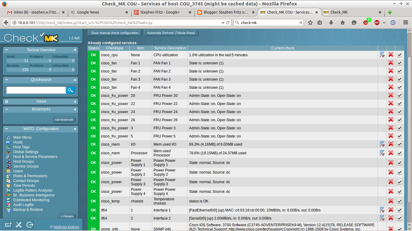
The discovery process is fairly thorough.  The illustration above depicts SNMP items discovered on a Cisco 3745 Router.  Discovery finds not just interfaces, but also fans, power supplies, CPU, memory and other counters.

By default, the SNMP Discovery process only searches for Ethernet and Frame Relay devices on all hosts.  If you have SONET or other interfaces, you must activate them from the Global Configuration screen.  That process is depicted in the video at the bottom of this article.

Parent relationship definitions are included for each host.  Parent relationships define topology -- as depicted above -- and also control Notifications.  A more thorough treatment discussion of Nagios/Icinga Logic, Alerts and Notifications is available in another blog article.  The illustration above depicts a NagVis-generated topology available from the Check-MK views.

Finally (at least as far as this article is concerned), OMD includes a preconfigured PNP4Nagios installation.  As soon as a host is added the application processes service check results and begins graphing them.  Although not depicted, Check-MK includes its own Perf-O-Meter views that are small and effective overviews of counters.
The video below depicts OMD installation on Debian Wheezy, a rather simple process described above.

The video below depicts configuring OMD for monitoring eight Cisco routers and two Linux Layer 2 Switches using the Check-MK interface.

GNS3 - VitualBox Part 7: OSPF over Frame Relay Switches

An explanation of mapped and Inverse ARP Frame Relay configurations and how to implement OSPF over them.

Introduction

Frame Relay is a Non Broadcast Multiple Access (NBMA) technology.  It operates at Layer 2 -- Datalink -- of the OSI Networking Model and relies upon connected nodes (in this case Cisco routers) to implement Layer 3 and above (in this case, TCP/IP).  NBMA technologies do not support broadcast and multicast traffic.  OSPF uses multicast packets for LSAs.  Additional configuration is required to implement OSPF on Frame Relay switched networks.

Frame Relay Basics

In Ethernet networks, this is implemented with Media Access Control (MAC) addresses -- 12-hexadecimal digit unique identifiers typically "burned in" to the hardware by the manufacturer.  When two nodes on an Ethernet network, they translate Layer 3 (e.g. IP) addresses into Layer 2 (MAC) addresses using Address Resolution protocol.  The Ethernet devices (e.g. hubs and switches) and supporting hardware (e.g. cabling, wireless) determine the path and access at Layer 2.  This sequence operates dynamically because the end nodes and networks support Address Resolution Protocol (ARP), which maps Layer 3 IP addresses to Layer 2 MAC addresses.

Frame Relay does not operate at Layer 2 the same way Ethernet does.  Frame Relay uses Data Link Connection Identifiers (DLCIs) assigned to physical interfaces rather than MAC addresses.  The switched Frame Relay network manages connections between DLCIs with mappings -- associating one DLCI with a corresponding one.  DLCIs are typically assigned by the Internet Service Provider (ISP).  A pathway from one DLCI to a corresponding DLCI is a Virtual Circuit (VC).  For this example, a unique and unchanging DLCI and data path is assigned for each VC, creating a Permanent Virtual Circuit (PVC).  Although not demonstrated in this article, DLCIs and paths may be assigned dynamically to endpoints (analogous to dial-up networking) and the resulting VCs are Switched Virtual Circuits (SVCs).

Each PVC requires a unique DLCI-DLCI mapping on the Frame Relay switched network.  This implies other differences between Frame Relay and Ethernet Layer 2 technologies:  Frame Relay must be manually configured with one or more unique Layer 2 addresses while Ethernet is configured with (typically) permanent Layer 2 addresses and the switches establish endpoint connections automatically.  Each Frame Relay endpoint must have a unique DLCI assigned for each connection to another endpoint, so a single endpoint will have multiple DLCIs if it connect to more than one other endpoint.

Example Frame Relay Layer 2 Topologies

The illustration at the top of the page depicts the Layer 1 Physical topology -- each router has a single serial T-1 connection to a Frame Relay switch port.  There are many Layer 2 -- DLCI-DLCI PVC mappings -- that may be implemented.

Hub and Spoke Topology

A hub and spoke topology applicable to a Data Center to five Branch Offices is to create a PVC connection from each Branch Office to the Data Center.  This is implemented by assigning five DLCIs to the Data Center endpoint (port 1) mapped to a each of a single DLCI assigned to each Branch Office (ports 2 through 6).  There are a total of five PVCs.  The illustration above depicts the logical Layer 2 Frame Relay Hub and Spoke DLCI-DLCI PVC mappings.

The format of the DLCIs used in the GNS3 Frame Relay switch example is "<source port> 0 <destination port>.  DLCI 102 is assigned to the PVC from interface 1 to interface 2 and is mapped to the corresponding DLCI 201  assigned to the PVC from interface 2 to interface 1.

Mesh Topology

A mesh topology applicable to a Data Center and five Branch Offices is to create a PVC connection between every endpoint.  Each endpoint has five unique DLCIs and there are a total of 15 PVCs.  The illustration above depicts the logical Layer 2 Frame Relay Mesh DLCI-DLCI PVC mappings.

Establishing Router-To-Router Connections Over Frame Relay

Ethernet uses ARP to map IP to MAC addresses.  When an IP node establishes a connection to another IP node, it first consults its local ARP cache (list of IP address to MAC adress mappings).  If there is no corresponding IP address to MAC address mapping, it sends out an ARP broadcast packet to determine the MAC address to use.  Frame Relay, as an NBMA technology, does not support broadcast packets.

Lacking broadcast support, establishing router-to-router IP connections over Frame Relay connections is a different process.

Manual IP Address-to-DCLI Mappings

Cisco IOS provides commands to manually map IP addresses to DLCIs.  Two important ones are frame-relay map and frame-relay interface-dlci.

Addresses Assigned to the Physical Interface

When an IP address is assigned to the physical serial interface (e.g. s0/0, s0/1, s1/0, etc.), Cisco IOS recognizes the assigned DLCIs in much the same way operating systems recognize Ethernet MAC addresses.  That is, the Cisco IOS on the router already has a mapping for its local DLCI assigned by the ISP to its physical interface.  However, it lacks a DLCI to remote IP address mapping (analogous to Ethernet's ARP cache).  This mapping may be established by manually specifying the remote IP address associated with the local DLCI using the frame-relay map command, whose syntax is:

frame-relay map <protocol> <destination IP address> <local DLCI> <option>

The goal is to support OSPF over the link and NBMA networks do not support broadcasts.  The operating system must specify that broadcast packets are forwarded to this DLCI, at which point the Frame Relay switched network delivers it to the corresponding DLCI and receiving device accepts the packet.  To do so, add the "broadcast" option to each configuration.  For example:

On Router 1:

frame-relay map ip 192.168.0.2 102 broadcast

On Router 2:

frame-relay map ip 192.168.0.1 201 broadcast

A complete example, mapping Router 1 with IP address 192.168.0.1/30 and DLCI 102 to Router 2 with IP address 192.168.0.2/30 and DLCI 201, is:

On Router 1:

config t
interface s0/0
no shutdown
ip address 192.168.0.1 255.255.255.252
encapsulation frame-relay
frame-relay map ip 192.168.0.2 102 broadcast

On Router 2:

config t
interface s0/0
no shutdown
ip address 192.168.0.2 255.255.255.252
encapsulation frame-relay
frame-relay map ip 192.168.0.1 201 broadcast

Addresses Assigned to Logical Subinterfaces

Logical subinterfaces (e.g. s0/0.1, s0/0.2, etc.) operate differently than physical interfaces.  They are logical devices created by the Cisco IOS, not physical ones recognized by the Cisco IOS.  One implication of this is that subinterfaces do not recognize any of the DLCIs assigned to their parent physical interfaces.  Before mapping remote IP addresses to local DLCIs, the subinterface must first have one or more DLCIs from the parent physical interface assigned to the logical subinterface.  Using the example above:

On Router 1:

config t
interface s0/0
no shutdown
encapsulation frame-relay
interface s0/0.1multipoint
ip address 192.168.0.1 255.255.255.252
frame-relay interface-dlci 102
frame-relay map ip 192.168.0.2 102 broadcast

On Router 2:

config t
interface s0/0
no shutdown
encapsulation frame-relay
interface s0/0.1 multipoint
ip address 192.168.0.2 255.255.255.252
frame-relay interface-dlci 201
frame-relay map ip 192.168.0.1 201 broadcast

Inverse ARP IP Address-To-DLCI Mappings

Frame Relay Inverse ARP is another way to map addresses.  ARP translates Layer 3 IP addresses to Layer 2 MAC addresses; Inverse ARP (as the name implies) translates Layer 2 DLCI addresses to Layer 3 IP addresses.  In operation, when a router requests a remote IP address, it sends Inverse ARP packets by matching the associated network and using any local IP addresses to decide where to send it.  It then sends the Inverse ARP packets to every DLCI mapped to candidate IP addresses.  On the receiving devices, the receiving DLCI that corresponds to the requested remote IP address responds, creating the PVC and DLCI-IP address mappings.

Consider the section above explaining how physical and logical interfaces interact with Cisco IOS.  When an IP address is assigned to a physical interface, the corresponding DLCIs are available to IOS.  However, when an IP address is assigned to a logical subinterface, there is no DLCI mapping until one is specified.  So, Inverse ARP works by default on physical interfaces as soon as an IP address is assigned.  Inverse ARP will not work on a logical subinterface until both an IP Address and DLCI assigned to the parent physical interface are assigned.  In fact, the frame-relay map command is disallowed on subinterfaces because if it is point-to-point because there is only one possible destination DLCI; multipoint subinterfaces still require mappings.

Once properly configured for Inverse ARP, the IP Address - DLCI mappings will be configured upon the router requesting the remote IP address.  Pinging the remote address will trigger the Inverse ARP request and dynamic DLCI mappings created.

Configuring OSPF over Frame Relay

The OSPF network type, by default, for frame relay is non-broadcast.  To manually set the OSPF network type to broadcast:

config t
interface s0/0
ip ospf network broadcast

At that point, the two routers will form an adjacency.

Optionally, you may manually specify the IP Address of neighboring routers using the neighbor command. 

The video below illustrates how to configure the above OSPF over Frame Relay options.

GNS3 - VitualBox Part 6: Stub, Totally Stubby and Not-So-Stubby OSPF Areas

An explanation of the various types of OSPF Stub Areas and demonstrations of how to configure Stub, Totally Stubby and Totally NSSA Areas.

 

Introduction

OSPF Stub Areas restrict the number and types of routing table updates -- Link State Advertisements -- they accept, limiting the amount of overall network topology detail they must maintain in their routing tables and link state databases.  A common (but by no means mandatory) implementation of Stub Areas is an OSPF Area that has only one ABR for all traffic between the Area and the rest of the Autonomous System.

OSPF Link State Advertisement Types

OSPF routers maintain a routing table and link state database by communicating topology information using Link State Advertisements (LSAs).  There are different types of LSAs; this article examines the six relevant to Stub Areas.

Type 1 - Router LSA

Type 1 - Router LSA - the router announces its presence and lists the links and metrics to other routers or networks in (and only within) its own area.  The link-state ID of the Type 1 LSA is the originating router ID.

Type 2 - Network LSA

Type 2 - Network LSA - the Area's designated router (DR) on a broadcast segment (e.g. Ethernet) lists the router IDs in broadcast domain. Type 2 LSAs are flooded across their own area only. The link-state ID of the Type 2 LSA is the IP interface address of the DR.

Type 3 - Summary LSA

Type 3 - Summary LSA - an Area Border Router (ABR) summarizes information about an Area and sends it to other attached Areas.  Summarization provides scalability by aggregating contiguous networks information into a single address/mask entry.  For instance, all of the individual networks in the 172.16.0.0 - 172.16.31.255 range may be summarized as 172.16.0.0 / 255.240.0.0 The link-state ID is the destination network number for Type 3 LSAs.

Type 4 - ASBR-Summary LSA

Type 4 - ASBR-Summary LSA - support Type 5 - External LSAs (see below).  Type 5 External LSAs list routes imported from external systems and are flooded to all areas in the OSPF Domain.  However, accurate next-hop information may not be available for other areas in the OSPF Domain with the Type 4 ASBR-Summary LSA which includes information specific to the ASBR advertising the routes.  The link-state ID is the router ID of the described ASBR for Type 4 LSAs.

Type 5 - External LSA

Type 5 - External LSA - provide routes imported into OSPF from other routing protocols. They are flooded to all areas unchanged (except stub and NSSA areas).  The link-state ID of the Type 5 LSA is the external network number.

Type 7 - NSSA External LSAs

Type 7 - NSSA External LSAs are specific to Not-So-Stubby-Areas (NSSA), which -- like Stub and Totally Stubby Areas -- do not receive external routes from ABRs.  Unlike Stub Areas, NSSA Areas may have links to external routing protocols. NSSA Areas use Type 7 LSAs to tell their ABRs about these external routes, which the Area Border Router then translates to type 5 external LSAs and floods as normal to the rest of the OSPF network.

OSPF Stub Area Types

The illustration above depicts the important differences between the four types of Stub Areas, the types of LSAs they use and relations to external routing protocols.  The most important concepts of stubby areas is understanding how they treat Type 3 Summary and Type 5 External LSAs.  In the NSSA area types, Type 7 NSSA External LSAs operate only within the NSSA Area, but are translated at border routers into Type 5 External LSAs.

Stub Areas

Stub Areas receive route summaries from the ABR via Type 3 Summary LSAs, providing information about networks in other Areas in the Autonomous System.  They also receive a default route.  They do not receive Type 5 External LSAs that provide information about routes external to the OSPF Autonomous System.

Totally Stubby Areas

Totally Stubby Areas receive neither Type 5 External LSAs nor Type 3 Summary LSAs from the ABR and lack both routes external to the OSPF Autonomous System and summary information about the networks in other Areas in the Autonomous System.  They are only aware of routes within their own Area and reach others through a default route, typically handled by the ABR.

Not-So-Stubby Areas

Not-So-Stubby Areas (NSSAs) differ from Stub and Totally Stubby Areas by including external routes (in the illustration above injected from EIGRP by and ASBR in the NSSA).  They are stubby with respect to the OSPF Autonomous System n that they do not receive Type 5 External LSAs but do receive Type 3 Summary LSAs from the ABR.  They differ significantly from Stub and Totally Stubby Areas in that they use Type 7 LSAs to advertise their external routes to the ABR, which then floods them to the OSPF Autonomous System as Type 5 External LSAs.  NSSAs differ from the other three types of Stub Areas in that they do not automatically assign default routes; these must be manually configured on the ABR.

Totally Not-So-Stubby Areas

Totally Not-So-Stubby Areas (Totally NSSAs) operate much like NSSAs with two important differences:  they receive neither Type 3 Summary nor Type 5 External LSAs (and thus do not have external routes) and do automatically assign default routes.

Configuring Stub and Totally Stub Areas

The illustrations at the beginning of this article depicts a network with several potential Stub Areas.  One, however, is not:  10.64.0.0.  This OSPF Area is a Transit Area providing a virtual link (see Part 5 of this series) to Backbone Area 0.0.0.0 for Area 10.72.0.0.  Area 10.72.0.0 is a WAN Border Router (10.64.0.0-10.72.0.0) serving Cisco 2691 Branch Office routers.  This is a good candidate for limiting the detail of routing information it maintains (the Link State Databases) by configuring it as a Stub or Totally Stubby Area.

Each router in the area must be configured with the following OSPF statement to create a Stub Area:

area 10.72.0.0 stub

This statement blocks Type 5 - External LSAs from Area 10.72.0.0.  However, notice the topology: there are no external routing protocols injecting routes into the OSPF Autonomous System.  Specifically, the ASBRs are simply Debian Linux Gateways with an external static route to the wireless router.  This will be apparent when comparing the Links State Databases on routers in Area 10.72.0.0 before and after -- there is no change.

Reducing the size of the Link State Databases in Area 10.72.0.0 in this system requires configuring it as a Totally Stubby Area.  Each router in the area must be configured with the following OSPF statement to create a Totally Stubby Area:

area 10.72.0.0 stub no-summary

This statement also blocks Type 3 - Summary LSAs from Area 10.72.0.0.  Now the change in this system is noticeable -- summary routes to other OSPF Areas are no longer listed in the Link State Databases, which now contain only routes within Area 10.72.0.0 and a default route.

The video below illustrates configuring area 10.72.0.0 as a Stub and then Totally Stubby Area.

Configuring Totally NSSA Areas

NSSA and Totally NSSA Areas are a difficult topic.  A simplified topology is warranted for clarity.  The illustration aboce is the topology that will be used in this section.

NSSA and Totally NSSA Areas are stubby with respect to OSPF, but connected to external routes and routing protocols.  Since Stub and Totally Stubby Areas do not accept Type 5 External LSAs, such an area would no longer inject external routes into OSPF.  NSSA and Totally NSSA Areas handle exteral routes using Type 7 NSSA External LSAs.  These LSAs inject external routes from the NSSA ASBR into the NSSA Area; the NSSA ABR then translates the Type 7 NSSA External LSAs into Type 5 External LSAs and floods the OSPF AS with the external routes.

Redistributing OSPF and External Routes

The first step in configuring a NSSA or Totally NSSA Area is to assure the external routing protocol and OSPF are exchanging information correctly.  The ASBR in this example (COU_ASBR) is already running OSPF and RIP.  It is the only router in the topology that is aware of all routes because it is not configured to redistribute.  The following commands enable redistribution of OSPF routes into RIP and RIP routes into OSPF:

router ospf 1
redistribute rip subnets

router rip
redistribute ospf 1 metric 1

Once configured, the router redistributes the routes.  Checking OSPF routers, RIP routes 192.168.x.x are now present.  Checking RIP routers, the OSPF route 10.0.0.0/8 is now present.

Creating the Totally NSSA Area 10.0.0.0

On all routers in the 10.0.0.0 Area (COU_ABR, COU_ASBR and COU_IR), issue the command:

area 10.0.0.0 nssa no-summary

This command drops Type 3 Summary and Type 5 External LSAs while creating Type 7 NSSA LSAs for the connected RIP External System.  IRs now have no OSPF Summary or External routes, but do have Intra Area and RIP External routes.  The ABR and ASBR manage redistribution of RIP External routes into OSPF and OSPF routes into RIP.

Creating the Stub Area 10.64.0.0 and Totally Stubby Area 10.128.0.0

The two normal Areas 10.64.0.0 and 10.128.0.0 maintain OSPF Summary Routes (10.x.x.x) and RIP External Routes (192.168.x.x).  Converting them to Stub and Totally Stubby Areas further summarizes routing information.

Convert Area 10.64.0.0 into a Stub Area by issuing, on all area routers, the command:

area 10.64.0.0 stub

Once converted, the Stub Area no longer accepts Type 5 External LSAs (originating at the COU_ABR router) and rely upon the default gateway (PHL_ABR) to maintain external routes.  Although the external routes are no longer maintained by IRs, you may still ping addresses in the RIP External System (192.168.x.x) and get responses.

The Stub Area still maintains Intra Area routes and summary routes (10.x.x.x) for OSPF AS Areas.


Convert Area 10.128.0.0 into a Totally Stubby Area by issuing, on all area routers, the command:

area 10.128.0.0 stub no-summary

Once converted, the Totally Stubby Area no longer accepts Type 3 Summary and Type 5 External LSAs (originating at the COU_ABR router) and rely upon the default gateway (PHL_ABR) to all but Intra Areal routes.  Although the routes are no longer maintained by IRs, you may still ping addresses in the OSPF AS (10.x.x.x) and RIP External System (192.168.x.x) and get responses.

The video below illustrates configuring Area 10.0.0.0 as Totally NSSA, Area 10.64.0.0 as Stub and 10.128.0.0 as Totally Stubby.